Introduction
GoDaddy has an automated service to give you the appraisal for a domain name on the secondary market. The domain name value prediction is powered by a deep learning model that we described in a past blog post. Now, another question that people may be curious about is: how confident is the model for that prediction? Can we quantify the uncertainty of the prediction? The answer is, YES! Using a prediction interval, we can quantify the uncertainty of a regression problem. Instead of predicting a single value, one can predict a range of possible values, which we call a prediction interval. If the model is uncertain, it will give a larger prediction interval; if the model is confident about the prediction, it will give a tighter prediction interval. Let’s take the domain appraisal problem as an example. A normal regression model gives a single prediction for a domain name. ThaiRestaurant.com might be predicted as $9,463. With prediction intervals, we instead have a range of predictions. For example, we might get a range from $9,000 to $10,000 for the same domain name. If the model is less certain about the prediction, the range can be larger, and the prediction interval may instead be $5,000 to $15,000. To dive more deeply into this topic, the GoDaddy machine learning team investigated this prediction interval problem and wrote a paper based on findings. In our paper, Tight Prediction Intervals Using Expanded Interval Minimization, we were curious to see if there was a better way to develop a model that would output prediction intervals which are meaningful and precise. The following sections of this post summarize our approach and the results.
Prediction Interval Evaluation
An essential first question for developing prediction intervals is how to evaluate them? This is a critical question since we need to know how to compare the performance of different prediction interval models. For a regression model that outputs a single prediction, we can directly compare the difference between the prediction and the true value. The smaller the difference, the better the regression model is. The assessment for prediction interval models is very different from the regression model assessment. A good prediction interval should first contain the actual value, and second, it should be tight. If we have an infinite prediction interval, it will cover the actual value, but it provides no valuable information to users. In the paper, we use two established metrics to measure the performance of the prediction interval model. First is the Prediction Interval Coverage Probability (PICP), which is the percentage of the time the prediction interval covers the actual value in a holdout set. Since we want to make sure that the prediction interval will cover the true value, the higher the PICP the better. However, using only PICP will not be enough since we can achieve 100% PICP (all prediction intervals will cover the true value) by setting the prediction interval to be infinity. Therefore, the second metric is the Mean Prediction Interval Width (MPIW) to measure the average size of all prediction intervals. In general, we want the model to have high PICP (typically reaching some threshold such as 80%) while maintaining a low MPIW. Now you may have a question: how can we know if a model is better than another model if the PICP is larger but the MPIW is also larger? We can put all the models on even ground by linearly scaling them to hit a given PICP target exactly. This allows us to compare each MPIW directly, with the smaller MPIW being better. For example, if the PICP for a given model is 76% and the target PICP is 80%, we will expand the prediction intervals (which makes the MPIW larger) to hit exactly 80%. On the other hand, if the PICP for a given model is 85%, we will shrink the prediction intervals to hit 80% PICP. After all the models we want to compare hit the same PICP target, we can compare the MPIW to check which model is the best.
Traditional Techniques
Before we dive into our new technique, let’s first discuss existing techniques to construct a prediction interval model from related literature. The first and most common way to construct prediction intervals is to predict the variance directly. We can view the prediction interval to be constructed by a point of estimation plus and minus a multiple of the predicted standard deviation (which is the square root of the variance). If we are less certain, the variance will be higher; if we’re more certain, the variance will be smaller, which results in smaller prediction intervals. Both the Maximum likelihood estimation and the Ensemble method are techniques trying to predict the variance directly. We also include the quantile regression method, and a naive baseline fixed bound method so that we can compare all these different techniques with our proposed method.
Fixed Bound Method
The fixed bounds method is a naive baseline so we can get a floor of performance that can be achieved with minimal effort. The technique trains a regression model to predict the true value then adds and subtracts a fixed percentage of that prediction value. For example, if the prediction is 3,000 and the fixed percentage is set to 30%, we can then construct a prediction interval with the lower bound to be 3000-(30%3000) and the upper bound to be 3000+(30%3000).
Maximum Likelihood Estimation
For the maximum likelihood method, we directly build two neural networks. The first neural network predicts the true value (like the $9,483 prediction for thairestaurant.com domain name), and the the second neural network predicts the absolute error of the first model, otherwise known as the variance. For example, if the variance prediction for thairestaurant.com might be $3,000, the prediction interval predicted by Maximum Likelihood estimation would be $6,483 to $12,483.
Ensemble Method
For the ensemble method, we build multiple neural network models that predict the true value and use the outputs from those neural network models to construct the prediction interval. Every neural network is trained on a subsample of the full dataset so, those models will be slightly different. We then take the average of the predictions from those neural networks to be the point of estimation and calculate the variance of those predictions to be the estimation of how confident the models are.
Quantile Regression Method
Quantile regression is a type of regression that predicts a specific quantile, such as the mean or 50%, of the data. Using quantile regression, we can construct prediction intervals by training two models to output different quantile of the prediction and thus construct an interval. For example, we can train one model to predict the 10th percentile of the prediction and another model to predict the 90th percentile of the prediction. Then we can construct a prediction interval using these two outputs.
Propose technique - Expanded Interval Minimization
In our paper, we present a new way to build a prediction interval model: Expanded Interval Minimization (EIM), a novel loss function for generating prediction intervals using neural networks. For every neural network model, we need to provide a loss function that we want it to learn to minimize. For example, for a regression problem, the loss function can be the mean square error - the mean of the squared difference between predictions and actual values. For the prediction interval problem, we want to hit the target PICP while minimizing the MPIW. We use the minibatch as a noisy estimate of the population PICP and MPIW. For every minibatch of data that feeds into the neural network, we scale the prediction interval to hit the fixed and given PICP like the way we discussed in the prediction interval evaluation section. After hitting the given PICP, we can calculate the MPIW and then use that as the loss function that we want the model to learn to minimize.
In practice, we found out that the EIM technique should use larger minibatches to get better results since the larger minibatches provide more stable estimates for the loss. Another improvement we did is to pretrain the EIM model on the fixed bound model. The pretraining process help mitigate early divergence issue when training the EIM model so the model can learn more efficient and effective.
Performance comparison
To compare the model performance, we applied the models on two real-world datasets. The first one is the aftermarket domain valuation dataset, which is the same dataset we used to build the domain name appraisal model as described in a previous blog post. The second one is the publicly available dataset - the million song dataset. This dataset is used to build the regression models based on the audio features of the songs to predict the release year. We set the target PICP (prediction interval coverage probability) to be 70%, 80%, and 90% and for each PICP, we calculate the scaled MPIW (mean prediction interval width) for each method. For a given PICP, the smaller the MPIW the better since it means that the prediction interval is tighter while we can expect the same accuracy from the model. Below are the performance tables for both dataset:
MPIW for Domain Valuation Dataset
| Method | Scaled MPIW to PICP=70% | Scaled MPIW to PICP=80% | Scaled MPIW to PICP=90% |
|---|---|---|---|
| Maximum Likelihood Method | 2488 | 2735 | 3689 |
| Ensemble Method | 1908 | 2480 | 3437 |
| EIM (trained with PICP=70%) | 1185 | 1889 | 3715 |
| EIM (trained with PICP=80%) | 1452 | 1692 | 3076 |
| EIM (trained with PICP=90%) | 2183 | 2362 | 2756 |
| Quantile 70 | 1804 | 2509 | 4802 |
| Quantile 80 | 1969 | 2402 | 3519 |
| Quantile 90 | 2108 | 2562 | 3485 |
| Fixed Bound Method | 2642 | 3077 | 3654 |
MPIW for Million Song Dataset
| Method | Scaled MPIW to PICP=70% | Scaled MPIW to PICP=80% | Scaled MPIW to PICP=90% |
|---|---|---|---|
| Maximum Likelihood Method | 15.5 | 18.93 | 27.37 |
| Ensemble Method | 16.92 | 19.91 | 25.74 |
| EIM (trained with PICP=70%) | 11.54 | 16.53 | 32.30 |
| EIM (trained with PICP=80%) | 12.18 | 15.00 | 26.23 |
| EIM (trained with PICP=90%) | 14.81 | 17.35 | 21.32 |
| Quantile 70 | 12.59 | 16.40 | 27.39 |
| Quantile 80 | 12.70 | 15.99 | 25.47 |
| Quantile 90 | 14.80 | 17.50 | 22.46 |
| Fixed Bound Method | 23.57 | 26.20 | 28.96 |
Based on the experiment results, we can see that for both real-world datasets, the EIM (Expanded Interval Minimization) method introduced here produces much tighter prediction intervals than other traditional techniques for different PICP targets. Since EIM and Quantile regression techniques can train the model for a specific PICP target, we see that it generally performs better than other techniques.

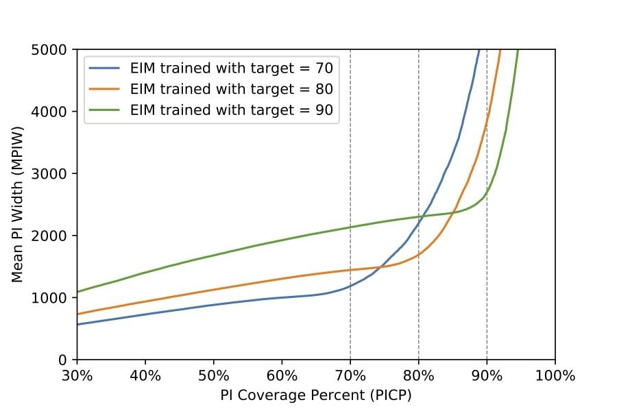
The above figure shows how different EIM models perform based on different target PICPs. For example, taking a look at 70% PICP EIM model (the blue line), you see that MPIW increases dramatically after reaching 70%. There are similar situations for 80% PICP EIM model and 90% PICP EIM model. The EIM model has specialized itself in the given PICP target.
Conclusion
Here in Godaddy Machine Learning, we keep up to date with the latest research, and in cases like this where existing techniques are insufficient, we try to expand the state of the art by developing novel machine learning techniques like EIM. The proposed Expanded Interval Minimization (EIM) method for prediction intervals has significantly better results than the existing techniques. While comparing to the next best technique, EIM produces 1.06x to 1.26x tighter prediction intervals given each target PICP (70%, 80%, and 90%). We hope that others will be able to use EIM to generate tighter prediction intervals and apply this technique to broader use cases.


